I used JetsonSeries(Nano, TX2), Ubuntu 18.04 Official image with root account.
This article quotes much from "
How to inspect a pre-trained TensorFlow model", and "
Speed up TensorFlow Inference on GPUs with TensorRT". And I consulted a lot of
official documents from NVODIA.
Brief introduction about TensorRT
NVIDIA® TensorRT™ is a deep learning platform that optimizes neural network models and speeds up for inference across GPU-accelerated platforms running in the datacenter, embedded and automotive devices. Jetson Series does not need to install TensorRT separately because the image is provided with TensorRT installed.
The following figure shows TensorRT defined as part high-performance inference optimizer and part runtime engine. It can take in neural networks trained on these popular frameworks, optimize the neural network computation, generate a light-weight runtime engine (which is the only thing you need to deploy to your production environment), and it will then maximize the throughput, latency, and performance on these GPU platforms.
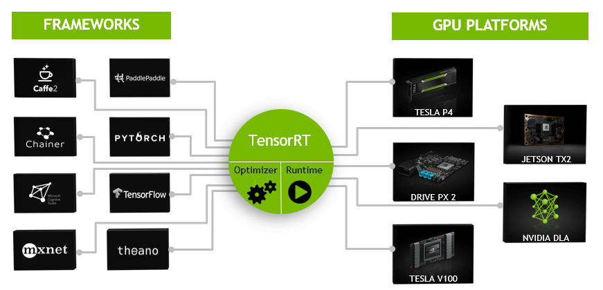
It is designed to work
in a complementary fashion with training frameworks such as
TensorFlow,
Caffe,
PyTorch,
MXNet, etc. It focuses
specifically on running an already trained network quickly and efficiently on a GPU for
the purpose of generating a result (a process that is referred to in various places as
scoring, detecting, regression, or inference).
Some training frameworks such as
TensorFlow have integrated
TensorRT so that it can be used to accelerate inference within the framework. Alternatively,
TensorRT can be used as a library within a user application. It
includes parsers for importing existing models from
Caffe,
ONNX, or
TensorFlow, and C++ and Python APIs for building models
programmatically.
TensorRT performs several important transformations and optimizations to the neural network graph (Fig 2). First, layers with unused output are eliminated to avoid unnecessary computation. Next, where possible convolution, bias, and ReLU layers are fused to form a single layer. Another transformation is horizontal layer fusion, or layer aggregation, along with the required division of aggregated layers to their respective output. Horizontal layer fusion improves performance by combining layers that take the same source tensor and apply the same operations with similar parameters. Note that these graph optimizations do not change the underlying computation in the graph: instead, they look to restructure the graph to perform the operations much faster and more efficiently.
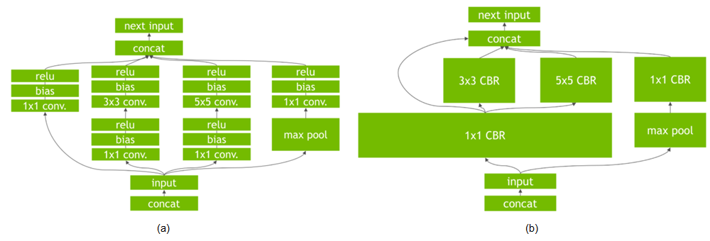
Figure 2 (a): An example convolutional neural network with multiple convolutional and activation layers. (b) TensorRT’s vertical and horizontal layer fusion and layer elimination optimizations simplify the GoogLeNet Inception module graph, reducing computation and memory overhead.Figure 2 (a): An example convolutional neural network with multiple convolutional and activation layers. (b) TensorRT’s vertical and horizontal layer fusion and layer elimination optimizations simplify the GoogLeNet Inception module graph, reducing computation and memory overhead.
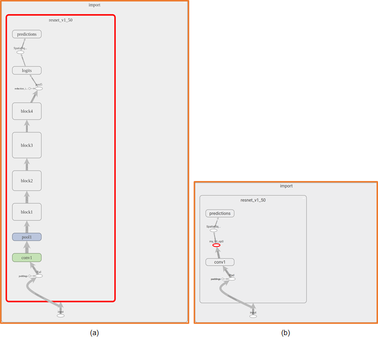
<Figure (a) ResNet-50 graph in TensorBoard (b) ResNet-50 after
TensorRT optimizations have been applied and the sub-graph replaced with
a TensorRT node.>
TensorRT optimizes the largest subgraphs possible in the TensorFlow
graph. The more compute in the subgraph, the greater benefit obtained from TensorRT. You want most of the graph optimized and replaced with the fewest
number of TensorRT nodes for best performance. Based on the operations in your
graph, it’s possible that the final graph might have more than one TensorRT
node.
With the TensorFlow API, you can specify the minimum number of nodes in a subgraph for
it to be converted to a TensorRT node. Any sub-graph with less than the
specified number of nodes will not be converted to TensorRT engines even if it
is compatible with TensorRT. This can be useful for models containing small
compatible sub-graphs separated by incompatible nodes, in turn leading to tiny TensorRT engines.
Tensorflow TensorRT Workflow
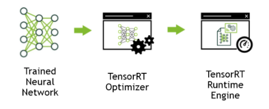
The following diagram shows the typical workflow in deploying a trained model for inference.
Figure 1. Deploying a trained model workflow.

In order to optimize the model using TF-TRT, the workflow changes to one of the following diagrams depending on whether the model is saved in SavedModel format or regular checkpoints. Optimizing with TF-TRT is the extra step that is needed to take place before deploying your model for inference.
Figure 2. Showing the SavedModel format.

Figure 3. Showing a Frozen graph.

Conversion API
The
original Python function
create_inference_graph that was used in
TensorFlow 1.13 and earlier is deprecated in TensorFlow >1.13 and removed in
TensorFlow 2.0.
So use TrtGraphConverter(tensorflow ver 1.x), TrtGraphConverterV2 (tensorflow ver 2.x).
TrtGraphConverter API
- input_saved_model_dir
Default value is None. This is the directory to load the
SavedModel which contains the input graph to transforms and is used only
when input_graph_def is None.
- input_saved_model_tags
Default value is None. This is a list of tags to load
the SavedModel.
- input_saved_model_signature_key
Default value is None. This is the key of the signature
to optimize the graph for.
- input_graph_def
Default value is None. This is a GraphDef object
containing a model to be transformed. If set to None,
the graph will be read from the SavedModel loaded from
input_saved_model_dir.
- nodes_blacklist
Default value is None. This is a list of node names to
prevent the converter from touching.
- session_config
Default value is None. This is the ConfigProto
used to create a Session. It's also used as a
template to create a TRT-enabled ConfigProto for
conversion. If not specified, a default ConfigProto is
used.
- max_batch_size
Default value is 1. This is the max size for the input
batch.
- max_workspace_size_bytes
Default value is 1GB. This is the maximum GPU temporary memory which the
TensorRT engine can use at execution time. This corresponds to the
workspaceSize parameter of
nvinfer1::IBuilder::setMaxWorkspaceSize().
- precision_mode
Default value is TrtPrecisionMode.FP32. This is one of
TrtPrecisionMode.supported_precision_modes() , in
other words, "FP32", "FP16" or "INT8" (lowercase is also supported).
- minimum_segment_size
Default value is 3. This is the minimum number of nodes
required for a subgraph to be replaced by
TRTEngineOp.
- is_dynamic_op
Default value is False. Whether to generate dynamic
TensorRT ops which will build the TensorRT network and engine at run
time.
- maximum_cached_engines
Default value is 1. This is the max number of cached
TensorRT engines in dynamic TensorRT ops. If the number of cached
engines is already at max but none of them can serve the input, the
TRTEngineOp will fall back to run the TensorFlow
function based on which the TRTEngineOp is created.
- use_calibration
Default value is
True. This argument is ignored if
precision_mode is not
INT8. If set
to
True, a calibration graph will be created to
calibrate the missing ranges. The calibration graph must be converted to
an inference graph by running calibration with
calibrate(). If set to
False,
quantization nodes will be expected for every tensor in the graph
(excluding those which will be fused). If a range is missing, an error
will occur.
Note: Accuracy may be negatively affected if there is a
mismatch between which tensors TensorRT quantizes and which tensors
were trained with fake quantization.
- use_function_backup
Default value is True. If set to True,
it will create a FunctionDef for each subgraph that is
converted to TensorRT op, and if TensorRT ops fail to execute at
runtime, it'll invoke that function as a fallback.
The main methods you can use in the
TrtGraphConverter class are the following:
- TrtGraphConverter.convert()
This method runs the conversion and returns the converted
GraphDef. The conversion and optimization that are
performed depends on the arguments passed to the constructor as
explained above.
In dynamic mode, where the TensorRT engines are built at runtime, this
method only segments the graph in order to separate the TensorRT
subgraphs, i.e. optimizing each TensorRT subgraph happens later during
runtime. In static mode, the optimization also happens in this method
and thus this method becomes time consuming.
- TrtGraphConverter.calibrate(fetch_names, num_runs, feed_dict_fn,
input_map_fn)
This method runs the INT8 calibration and returns the calibrated
GraphDef. This method should be called after
convert() in order to execute the calibration on
the converted graph. The method accepts the following arguments:
- fetch_names
A list of output tensor name to fetch during
calibration.
- num_runs
Number of runs of the graph during calibration.
- feed_dict_fn
A function that returns a dictionary mapping input names
(as strings) in the GraphDef to be calibrated to values
(e.g. Python list, NumPy
arrays, etc).One and only one of
feed_dict_fn and
input_map_fn should be
specified.
- input_map_fn
- A function that returns a dictionary mapping input names (as
strings) in the GraphDef to be calibrated
to Tensor objects. The values of the named input tensors in
the GraphDef to be calibrated will be
re-mapped to the respective Tensor values
during calibration. One and only one of
feed_dict_fn and
input_map_fn should be specified.
- TrtGraphConverter.save(output_saved_model_dir)
This method saves the converted graph as a
SavedModel.
TrtGraphConverterV2 API
- input_saved_model_dir
Default value is None. This is the directory to load the
SavedModel which contains the input graph to transforms.
- input_saved_model_tags
Default value is None. This is a list of tags to load the
SavedModel.
- input_saved_model_signature_key
Default value is None. This is the key of the signature to optimize
the graph for.
- conversion_params
Default value is
DEFAULT_TRT_CONVERSION_PARAMS. An instance of
namedtupleTrtConversionParams consisting the following items:
- rewriter_config_template
A template RewriterConfig proto used to create a TRT-enabled
RewriterConfig. If None, it will use a
default one.
- max_workspace_size_bytes
Default value is 1GB. The maximum GPU temporary memory which
the TensorRT engine can use at execution time. This corresponds to the
workspaceSize parameter of
nvinfer1::IBuilder::setMaxWorkspaceSize().
- precision_mode
Default value is TrtPrecisionMode.FP32. This is one of
TrtPrecisionMode.supported_precision_modes(), in other
words, FP32, FP16 or INT8
(lowercase is also supported).
- minimum_segment_size
Default value is 3. This is the minimum number of nodes
required for a subgraph to be replaced by TRTEngineOp.
- maximum_cached_engines
Default value is 1. This is the maximum number of cached
TensorRT engines in dynamic TensorRT ops. If the number of cached engines is
already at max but none of them can serve the input, the
TRTEngineOp will fall back to run the TensorFlow function
based on which the TRTEngineOp is created.
- use_calibration
Default value is
True. This argument is ignored if
precision_mode is not
INT8. If set to
True, a calibration graph will be created to calibrate the
missing ranges. The calibration graph must be converted to an inference graph
by running calibration with
calibrate(). If set to
False, quantization nodes will be expected for every tensor
in the graph (excluding those which will be fused). If a range is missing, an
error will occur.
Note: Accuracy may be negatively affected if there is a
mismatch between which tensors TensorRT quantizes and which tensors were
trained with fake quantization.
The main methods you can use in the
TrtGraphConverter class are the following:
- TrtGraphConverter.convert(calibration_input_fn)
This method runs the conversion and returns the converted TensorFlow function (note
that this method returns the converted GraphDef in TensorFlow 1.x).
The conversion and optimization that are performed depends on the arguments passed to
the constructor as explained above.
This method only segments the graph in order to separate the TensorRT subgraphs, i.e.
optimizing each TensorRT subgraph happens later during runtime (in TensorFlow 1.x this
behaviour depends on is_dynamic_mode but this argument is not
supported in TensorFlow 2.0 anymore; i.e. only is_dynamic_op=True is
supported).
This method has only one optional argument which should be used in case INT8
calibration is desired. The argument calibration_input_fn is a
generator function that yields input data as a list or tuple, which will be used to
execute the converted signature for INT8 calibration. All the returned input data
should have the same shape. Note that in TensorFlow 1.x, the INT8 calibration was
performed using the separate method calibrate() which is removed from
TensorFlow 2.0.
- TrtGraphConverter.build(input_fn)
This method optimizes the converted function (returned by convert())
by building TensorRT engines. This is useful in case the user wants to perform the
optimizations before runtime. The optimization is done by running inference on the
converted function using the input data received from the argument
input_fn. This argument is a generator function that yields input
data as a list or tuple.
- TrtGraphConverter.save
This method saves the converted function as a SavedModel. Note that
the saved TensorFlow model is still not optimized yet with TensorRT (engines are not
built) in case build() is not called
Conversion Example
If you have a frozen graph of your
TensorFlow model, you first need to load the frozen
graph file and parse it to create a deserialized
GraphDef. Then you can use
the
GraphDef to create a
TensorRT inference graph, for
example:
This example reads a tensorflow model and then converts it to a TensorRT model(trt_graph)
import tensorflow as tf
from tensorflow.python.compiler.tensorrt import trt_convert as trt
with tf.Session() as sess:
    # First deserialize your frozen graph:
    with tf.gfile.GFile(“/path/to/your/frozen/graph.pb”, ‘rb’) as f:
        frozen_graph = tf.GraphDef()
        frozen_graph.ParseFromString(f.read())
    # Now you can create a TensorRT inference graph from your
    # frozen graph:
    converter = trt.TrtGraphConverter(
     input_graph_def=frozen_graph,
     nodes_blacklist=['logits', 'classes']) #output nodes
    trt_graph = converter.convert()
    # Import the TensorRT graph into a new graph and run:
    output_node = tf.import_graph_def(
        trt_graph,
        return_elements=['logits', 'classes'])
    sess.run(output_node)
<https://docs.nvidia.com/deeplearning/frameworks/tf-trt-user-guide/index.html#using-frozengraph>
Be careful : Only use TrtGraphConverter with TensorFlow version 1.14 or later. In version 1.13 and earlier, use "create_inference_graph" function instead.
Everything except the nodes_blacklist(output nodes) seems to be find. What is the nodes_blacklist? And how can I find that?
To find this output node value, you must inspect the tensorflow model first. This value is the last node of the model.
Viewing the model in TensorBoard
To get the last node information, you need to view the pb file(frozen graph).
This is a simple python that creates log. Run this code to create the log files.
import argparse
import tensorflow as tf

parser = argparse.ArgumentParser(description='tf-model-conversion to TensorRT')
parser.add_argument('--model_dir', type=str, default='')
parser.add_argument('--log_dir', type=str, default='')
args = parser.parse_args()


with tf.Session() as sess:
    model_filename = args.model_dir
    with tf.gfile.GFile(model_filename, 'rb') as f:
        graph_def = tf.GraphDef()
        graph_def.ParseFromString(f.read())
        g_in = tf.import_graph_def(graph_def)
LOGDIR=args.log_dir
train_writer = tf.summary.FileWriter(LOGDIR)
train_writer.add_graph(sess.graph)
train_writer.flush()
train_writer.close()
<pb_viewer.py>
I'll use tf-pose-estimation example. Please see
my other article. Now there's a new log file in the ./logs directory that describes graph_opt.pb file.
# python3 pb_viewer.py --model_dir ./models/graph/cmu/graph_opt.pb --log_dir ./logs
# ls -al logs
total 204436
drwxr-xr-x  2 root root      4096 11월 25 23:16 .
drwxr-xr-x 16 root root      4096 11월 25 23:15 ..
-rw-r--r--  1 root root 209333789 11월 25 23:16 events.out.tfevents.1574691381.spytx-desktop
Now run Tensorboard like this. If successful, last log would be the URL of the tensorboard you started.
root@spytx-desktop:/work/src/pose_estimation/tf-pose-estimation# tensorboard --logdir=/work/src/pose_estimation/tf-pose-estimation/logs
.........
.........
TensorBoard 1.14.0 at http://spytx-desktop:6006/ (Press CTRL+C to quit)
Then access tensorboard from your desktop using a web browser. Because the log file is quite large, it may take a while for the browser screen to load.
When you first open the model in TensorBoard, you’ll just see one node called “import”. At the top right you’ll see “Subgraph: 276 nodes”, which is the hint that there is more to see.
You can double click on the “import” node and it will expand to show you the full graph. You’ll need to zoom out and scroll around to get it to fit nicely, but you should be able to see the full graph on one screen:
You can also zoom in and see the output node at the top of the screen:
In
my other article , I made python code like this. Outpur node value "Openpose/concat_stage7" comes from above picture.
# convert (optimize) frozen model to TensorRT model
your_outputs = ["Openpose/concat_stage7"]

start = time.time()
trt_graph = trt.create_inference_graph(
    input_graph_def=frozen_graph,# frozen model
    outputs=your_outputs,
    is_dynamic_op=True,
    minimum_segment_size=3,
    maximum_cached_engines=int(1e3),
    max_batch_size=1,# specify your max batch size
    max_workspace_size_bytes=2*(10**9),# specify the max workspace
    precision_mode="FP16") # precision, can be "FP32" (32 floating point precision) or "FP16"
Save the TensorRT model
Modify the directory of models, outputs for your purpose. This code is created to save the TensorRT model of my article "
Human Pose estimation using tensorflow"
import argparse
import sys, os
import time
import tensorflow as tf

ver=tf.__version__.split(".")
if(int(ver[0]) == 1 and int(ver[1]) <= 13):
#if tensorflow vereion <= 1.13.1 use this module
    print('tf Version <= 1.13')
    import tensorflow.contrib.tensorrt as trt
else:
#if tensorflow vereion > 1.13.1 use this module instead
    print('tf Version > 1.13')
    from tensorflow.python.compiler.tensorrt import trt_convert as trt


def get_frozen_graph(graph_file):
  """Read Frozen Graph file from disk."""
  with tf.gfile.FastGFile(graph_file, "rb") as f:
    graph_def = tf.GraphDef()
    graph_def.ParseFromString(f.read())
  return graph_def


parser = argparse.ArgumentParser(description='tf network model conversion to tensorrt')
parser.add_argument('--model', type=str, default='mobilenet_v2_small',
                        help='cmu / mobilenet_thin / mobilenet_v2_large / mobilenet_v2_small')
args = parser.parse_args()

model_dir = 'models/graph/'
frozen_name = model_dir + args.model + '/graph_opt.pb'
frozen_graph = get_frozen_graph(frozen_name)
print('=======Frozen Name:%s======='%(frozen_name));
# convert (optimize) frozen model to TensorRT model
your_outputs = ["Openpose/concat_stage7"]

start = time.time()

if(int(ver[0]) == 1 and int(ver[1]) <= 13):
    trt_graph = trt.create_inference_graph(
        input_graph_def=frozen_graph,# frozen model
        outputs=your_outputs,
        is_dynamic_op=True,
        minimum_segment_size=3,
        maximum_cached_engines=int(1e3),
        max_batch_size=1,# specify your max batch size
        max_workspace_size_bytes=2*(10**9),# specify the max workspace
        precision_mode="FP16") # precision, can be "FP32" (32 floating point precision) or "FP16"
else:
    converter =trt.TrtGraphConverter(
        input_graph_def=frozen_graph,# frozen model
        max_batch_size=1,
        precision_mode="FP16",
        minimum_segment_size=3,
        is_dynamic_op=True,
        nodes_blacklist=your_outputs)
    trt_graph = converter.convert()

elapsed = time.time() - start
print('Tensorflow model => TensorRT model takes : %f'%(elapsed));

#write the TensorRT model to be used later for inference
rt_name = model_dir + args.model + '/graph_opt_rt.pb'
with tf.gfile.FastGFile(rt_name , 'wb') as f:
    f.write(trt_graph.SerializeToString())
Wrapping up
After creating a log in the TensorFlow model, you can use the TensorBoard to find the final output node information. And use the TrtGraphConverter or create_inference_graph function to build a model for TensorRT using this information. I'll continue this story in the next article.